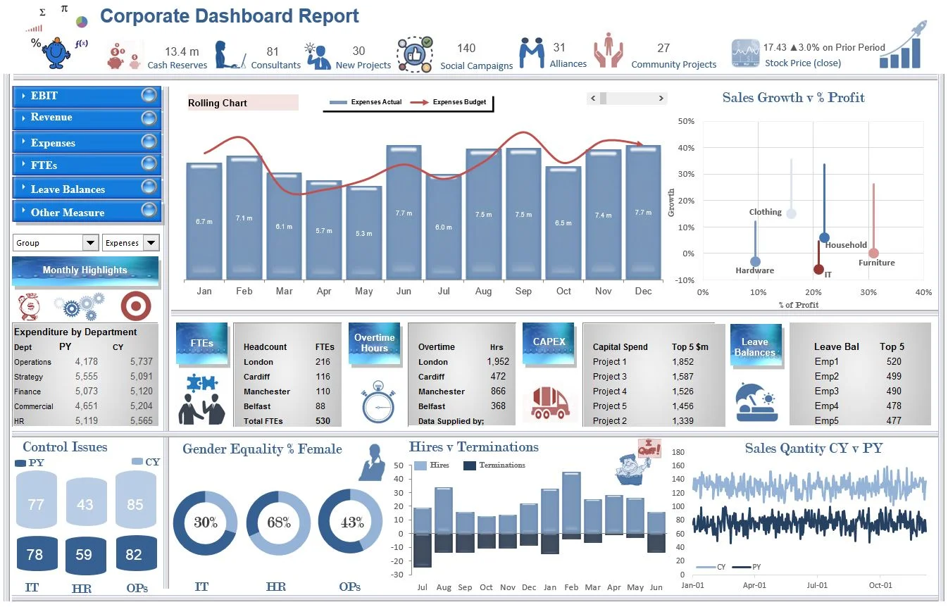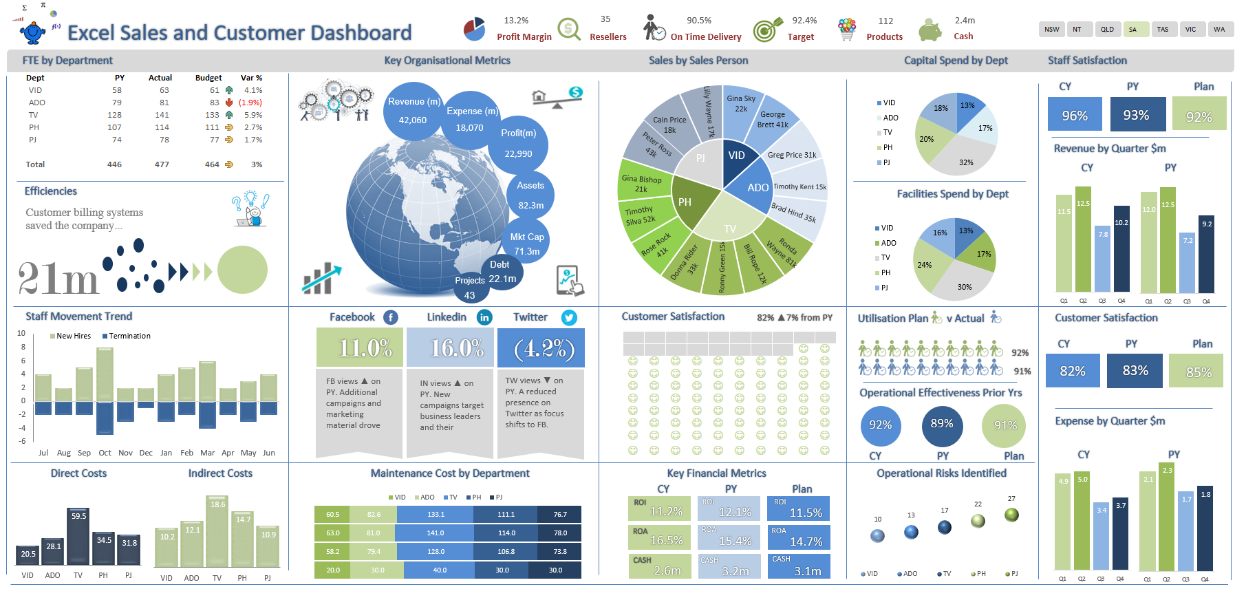
Excel Templates Dashboard
Excel Templates Dashboard - Excel has recently introduced a huge feature called dynamic arrays. I need help on my excel sheet. For example as simple as. Is there any direct way to get this information in a cell? I've got some cells that i have conditionally formatted to excel's standard 'bad' style (dark red text, light red fill). In your example you fix the. In another column i have cells that i have created a conditional formatting. It would mean you can apply textual functions like left/right/mid on a conditional basis without. I would like to use the =today () function in a table in excel. In a text about excel i have read the following: It would mean you can apply textual functions like left/right/mid on a conditional basis without. To convert them into numbers 1 or 0, do some mathematical operation. For example as simple as. Is there any direct way to get this information in a cell? I need help on my excel sheet. Then if i copied that. The dollar sign allows you to fix either the row, the column or both on any cell reference, by preceding the column or row with the dollar sign. And along with that, excel also started to make a substantial upgrade to their formula language. In most of the online resource i can find usually show me how to retrieve this information in vba. =sum(!b1:!k1) when defining a name for a cell and this was entered into the refers to field. If a1 = n/a then c1 = b1 else if a1 != n/a or has value(int) then c1 = a1*b1 To solve this problem in excel, usually i would just type in the literal row number of the cell above, e.g., if i'm typing in cell a7, i would use the formula =a6. And along with that, excel also started. Boolean values true and false in excel are treated as 1 and 0, but we need to convert them. And along with that, excel also started to make a substantial upgrade to their formula language. In a text about excel i have read the following: Then if i copied that. =sum(!b1:!k1) when defining a name for a cell and this. =sum(!b1:!k1) when defining a name for a cell and this was entered into the refers to field. To convert them into numbers 1 or 0, do some mathematical operation. In your example you fix the. Then if i copied that. I would like to use the =today () function in a table in excel. To convert them into numbers 1 or 0, do some mathematical operation. Is there any direct way to get this information in a cell? I need help on my excel sheet. In most of the online resource i can find usually show me how to retrieve this information in vba. However, once data has been entered into that table row,. To solve this problem in excel, usually i would just type in the literal row number of the cell above, e.g., if i'm typing in cell a7, i would use the formula =a6. In your example you fix the. Boolean values true and false in excel are treated as 1 and 0, but we need to convert them. In another. To convert them into numbers 1 or 0, do some mathematical operation. How can i declare the following if condition properly? =sum(!b1:!k1) when defining a name for a cell and this was entered into the refers to field. In another column i have cells that i have created a conditional formatting. In most of the online resource i can find. =sum(!b1:!k1) when defining a name for a cell and this was entered into the refers to field. Is there any direct way to get this information in a cell? For example as simple as. If a1 = n/a then c1 = b1 else if a1 != n/a or has value(int) then c1 = a1*b1 However, once data has been entered. Then if i copied that. I would like to use the =today () function in a table in excel. Is there any direct way to get this information in a cell? The dollar sign allows you to fix either the row, the column or both on any cell reference, by preceding the column or row with the dollar sign. And. Excel has recently introduced a huge feature called dynamic arrays. In another column i have cells that i have created a conditional formatting. And along with that, excel also started to make a substantial upgrade to their formula language. The dollar sign allows you to fix either the row, the column or both on any cell reference, by preceding the. =sum(!b1:!k1) when defining a name for a cell and this was entered into the refers to field. It would mean you can apply textual functions like left/right/mid on a conditional basis without. The dollar sign allows you to fix either the row, the column or both on any cell reference, by preceding the column or row with the dollar sign.. Excel has recently introduced a huge feature called dynamic arrays. If a1 = n/a then c1 = b1 else if a1 != n/a or has value(int) then c1 = a1*b1 To solve this problem in excel, usually i would just type in the literal row number of the cell above, e.g., if i'm typing in cell a7, i would use the formula =a6. In your example you fix the. Then if i copied that. However, once data has been entered into that table row, i would like it never to change dates again (effectively. To convert them into numbers 1 or 0, do some mathematical operation. For example as simple as. I need help on my excel sheet. In most of the online resource i can find usually show me how to retrieve this information in vba. =sum(!b1:!k1) when defining a name for a cell and this was entered into the refers to field. In a text about excel i have read the following: In another column i have cells that i have created a conditional formatting. Boolean values true and false in excel are treated as 1 and 0, but we need to convert them. I would like to use the =today () function in a table in excel. Is there any direct way to get this information in a cell?
Excel Dashboard Templates Empowering Data Visualization And Decision
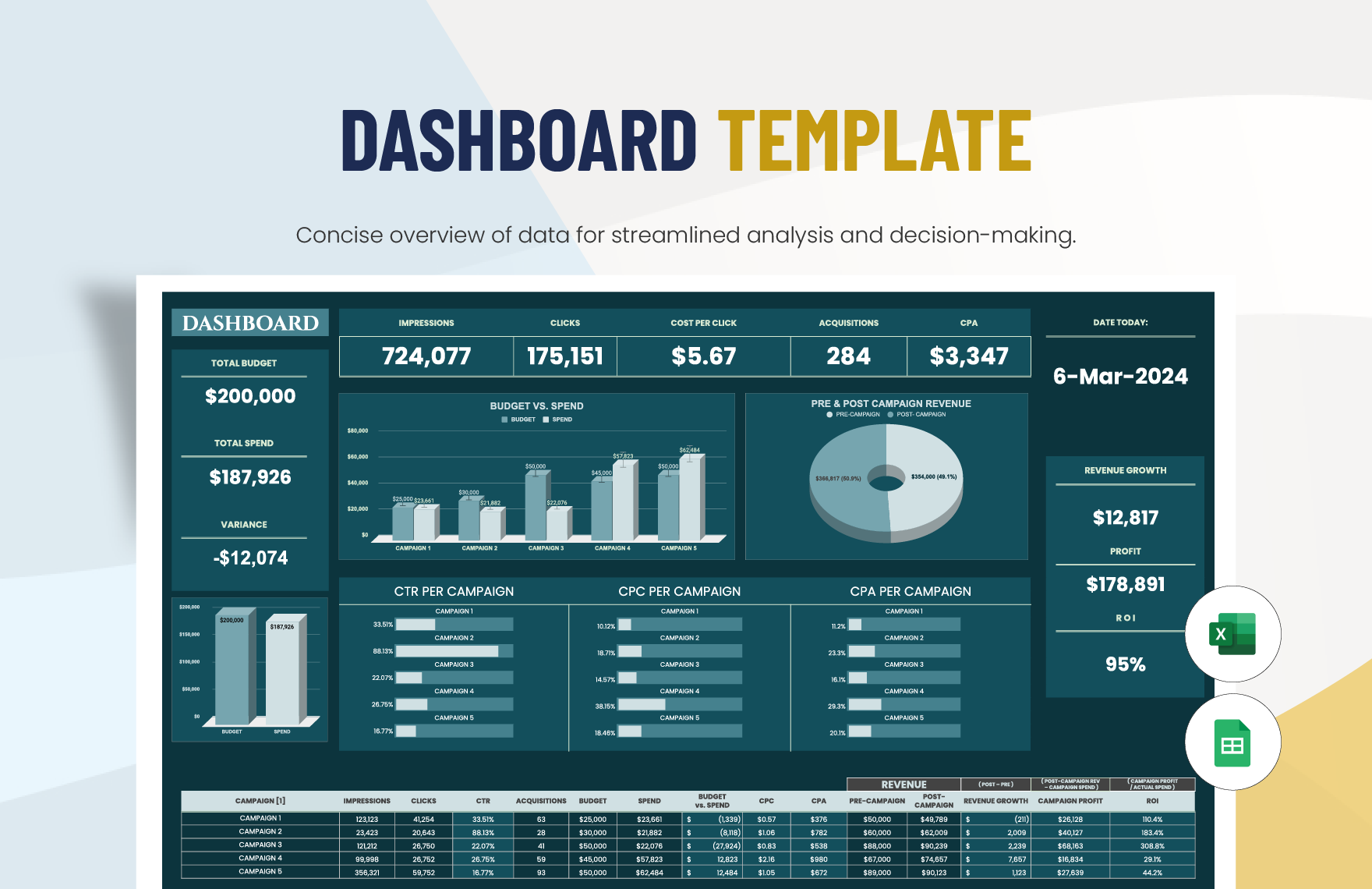
Dashboard Templates in Excel FREE Download
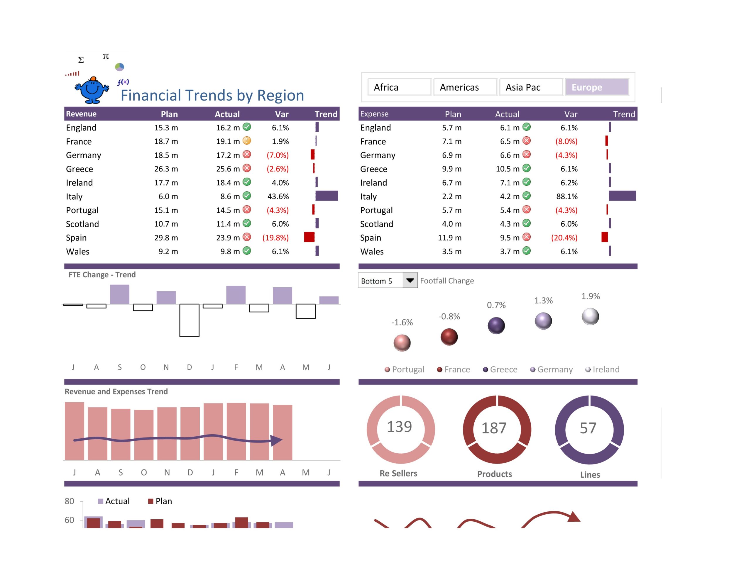
Free Excel Kpi Dashboard Templates Printable Form, Templates and Letter
5 Excel Project Dashboard Templates Excel Templates Excel Templates Riset

Kpi Excel Dashboard Templates

Ultimate Sales Performance Dashboard in Excel TheDataLabs
Free Kpi Dashboard Excel Template

Excel Kpi Dashboard Templates
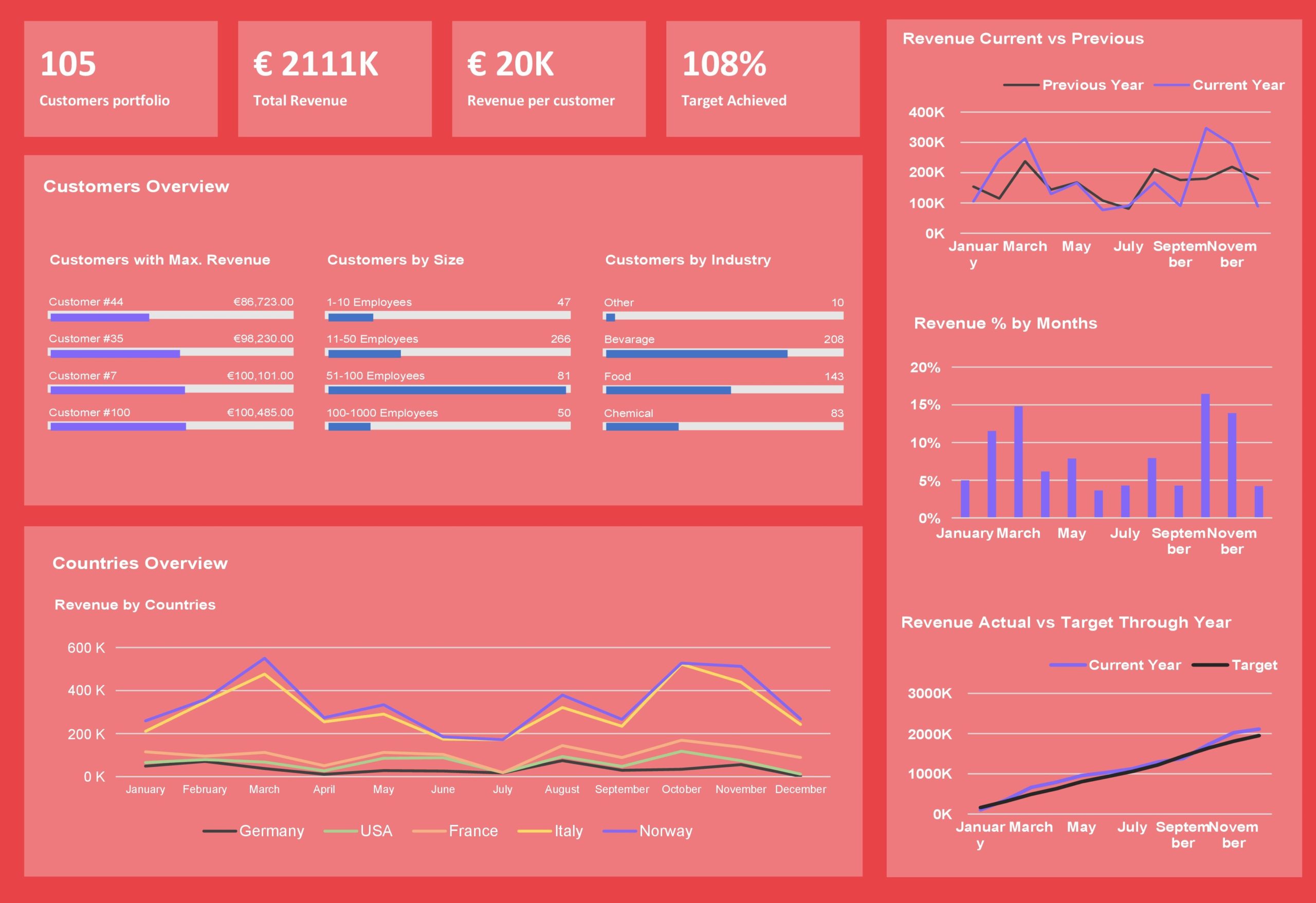
How To Show Dashboard In Excel
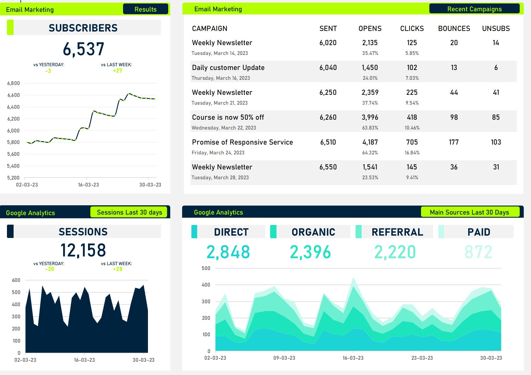
Hse Dashboard Excel Templates Free Free Printable
The Dollar Sign Allows You To Fix Either The Row, The Column Or Both On Any Cell Reference, By Preceding The Column Or Row With The Dollar Sign.
How Can I Declare The Following If Condition Properly?
I've Got Some Cells That I Have Conditionally Formatted To Excel's Standard 'Bad' Style (Dark Red Text, Light Red Fill).
And Along With That, Excel Also Started To Make A Substantial Upgrade To Their Formula Language.
Related Post: